User input file¶

The input file is organized in sections and keywords that can be of different type. Input keywords and sections are case-sensitive, while values are case-insensitive.

Section {
  keyword_1 = 1                         # int
  keyword_2 = 3.14                      # float
  keyword_3 = [1, 2, 3]                 # int array
  keyword_4 = foo                       # string
  keyword_5 = true                      # boolean
}

Valid options for booleans are true/false, on/off or yes/no. Single word strings can be given without quotes (be careful of special characters, like slashes in file paths). A complete list of available input keywords can be found in the User input reference.

Top section¶

The main input section contain four keywords: the relative precision \(\epsilon_{rel}\) that will be guaranteed in the calculation and the size, origin and unit of the computational domain. The top section is not specified by name, just write the keywords directly, e.g

world_prec = 1.0e-5                     # Overall relative precision
world_size = 5                          # Size of domain 2^{world_size}
world_unit = bohr                       # Global length unit
world_origin = [0.0, 0.0, 0.0]          # Global gauge origin

The relative precision sets an upper limit for the number of correct digits you are expected to get out of the computation (note that \(\epsilon_{rel}=10^{-6}\) yields \(\mu\) Ha accuracy for the hydrogen molecule, but only mHa accuracy for benzene).

The computational domain is always symmetric around the origin, with total size given by the world_size parameter as \([2^n]^3\), e.i. world_size = 5 gives a domain of \([-16,16]^3\). Make sure that the world is large enough to allow the molecular density to reach zero on the boundary. The world_size parameter can be left out, in which case the size will be estimated based on the molecular geometry. The world_unit relates to all coordinates given in the input file and can be one of two options: angstrom or bohr.

Note

The world_size will be only approximately scaled by the angstrom unit, by adding an extra factor of 2 rather than the appropriate factor of ~1.89. This means that e.g. world_size = 5 (\([-16,16]^3\)) with world_unit = angstrom will be translated into \([-32,32]^3\) bohrs.

Precisions¶

MRChem uses a smoothed nuclear potential to avoid numerical problems in connection with the \(Z/|r-R|\) singularity. The smoothing is controlled by a single parameter nuc_prec that is related to the expected error in the energy due to the smoothing. There are also different precision parameters for the construction of the Poisson and Helmholtz integral operators.

Precisions {
  nuclear_prec = 1.0e-6                 # For construction of nuclear potential
  poisson_prec = 1.0e-6                 # For construction of Poisson operators
  helmholtz_prec = 1.0e-6               # For construction of Helmholtz operatos
}

By default, all precision parameters follow world_prec and usually don’t need to be changed.

Printer¶

This section controls the format of the printed output file (.out extension). The most important option is the print_level, but it also gives options for number of digits in the printed output, as well as the line width (defaults are shown):

Printer {
  print_level = 0                       # Level of detail in the printed output
  print_width = 75                      # Line width (in characters) of printed output
  print_prec = 6                        # Number of digits in floating point output
}

Note that energies will be printed with twice as many digits. Available print levels are:

print_level=-1 no output is printed
print_level=0 prints mainly properties
print_level=1 adds timings for individual steps
print_level=2 adds memory and timing information on OrbitalVector level
print_level=3 adds details for individual terms of the Fock operator
print_level=4 adds memory and timing information on Orbital level
print_level>=5 adds debug information at MRChem level
print_level>=10 adds debug information at MRCPP level

MPI¶

This section defines some parameters that are used in MPI runs (defaults shown):

MPI {
  bank_size = -1                        # Number of processes used as memory bank
  numerically_exact = false             # Guarantee MPI invariant results
  share_nuclear_potential = false       # Use MPI shared memory window
  share_coulomb_potential = false       # Use MPI shared memory window
  share_xc_potential = false            # Use MPI shared memory window
}

The memory bank will allow larger molecules to get though if memory is the limiting factor, but it will be slower, as the bank processes will not take part in any computation. For calculations involving exact exchange (Hartree-Fock or hybrid DFT functionals) a memory bank is required whenever there’s more than one MPI process. A negative bank size will set it automatically based on the number of available processes. For pure DFT functionals on smaller molecules it is likely more efficient to set bank_size = 0, otherwise it’s recommended to use the default. If a particular calculation runs out of memory, it might help to increase the number of bank processes from the default value.

The numerically_exact keyword will trigger algorithms that guarantee that the computed results are invariant (within double precision) with respect to the number or MPI processes. These exact algorithms require more memory and are thus not default. Even when the numbers are not MPI invariant they should be correct and identical within the chosen world_prec.

The share_potential keywords are used to share the memory space for the particular functions between all processes located on the same physical machine. This will save memory but it might slow the calculation down, since the shared memory cannot be “fast” memory (NUMA) for all processes at once.

Basis¶

This section defines the polynomial MultiWavelet basis

Basis {
  type = Interpolating                  # Legendre or Interpolating
  order = 7                             # Polynomial order of MW basis
}

The MW basis is defined by the polynomial order \(k\), and the type of scaling functions: Legendre or Interpolating polynomials (in the current implementation it doesn’t really matter which type you choose). Note that increased precision requires higher polynomial order (use e.g \(k = 5\) for \(\epsilon_{rel} = 10^{-3}\), and \(k = 13\) for \(\epsilon_{rel} = 10^{-9}\), and interpolate in between). If the order keyword is left out it will be set automatically according to

\[k=-1.5*log_{10}(\epsilon_{rel})\]

The Basis section can usually safely be omitted in the input.

Molecule¶

This input section specifies the geometry (given in world_unit units), charge and spin multiplicity of the molecule, e.g. for water (coords must be specified, otherwise defaults are shown):

Molecule {
  charge = 0                            # Total charge of molecule
  multiplicity = 1                      # Spin multiplicity
  translate = false                     # Translate CoM to world_origin
$coords
O   0.0000     0.0000     0.0000        # Atomic symbol and coordinate
H   0.0000     1.4375     1.1500        # Atomic symbol and coordinate
H   0.0000    -1.4375     1.1500        # Atomic symbol and coordinate
$end
}

Since the computational domain is always cubic and symmetric around the origin it is usually a good idea to translate the molecule to the origin (as long as the world_origin is the true origin).

WaveFunction¶

Here we give the wavefunction method and whether we run spin restricted (alpha and beta spins are forced to occupy the same spatial orbitals) or not (method must be specified, otherwise defaults are shown):

WaveFunction {
  method = <wavefunction_method>        # Core, Hartree, HF or DFT
  restricted = true                     # Spin restricted/unrestricted
}

There are currently four methods available: Core Hamiltonian, Hartree, Hartree-Fock (HF) and Density Functional Theory (DFT). When running DFT you can either set one of the default functionals in this section (e.g. method = B3LYP), or you can set method = DFT and specify a “non-standard” functional in the separate DFT section (see below). See User input reference for a list of available default functionals.

Note

Restricted open-shell wavefunctions are not supported.

DFT¶

This section can be omitted if you are using a default functional, see above. Here we specify the exchange-correlation functional used in DFT (functional names must be specified, otherwise defaults are shown)

DFT {
  spin = false                          # Use spin-polarized functionals
  density_cutoff = 0.0                  # Cutoff to set XC potential to zero
$functionals
<func1>     1.0                         # Functional name and coefficient
<func2>     1.0                         # Functional name and coefficient
$end
}

You can specify as many functionals as you want, and they will be added on top of each other with the given coefficient. Both exchange and correlation functionals must be set explicitly, e.g. SLATERX and VWN5C for the standard LDA functional. For hybrid functionals you must specify the amount of exact Hartree-Fock exchange as a separate functional EXX (EXX 0.2 for B3LYP and EXX 0.25 for PBE0 etc.). Option to use spin-polarized functionals or not. Unrestricted calculations will use spin-polarized functionals by default. The XC functionals are provided by the XCFun library.

Properties¶

Specify which properties to compute. By default, only the ground state SCF energy as well as orbital energies will be computed. Currently the following properties are available (all but the dipole moment are false by default)

Properties {
  dipole_moment = true                  # Compute dipole moment
  quadrupole_moment = false             # Compute quadrupole moment
  polarizabiltity = false               # Compute polarizability
  magnetizability = false               # Compute magnetizability
  nmr_shielding = false                 # Compute NMR shieldings
  geometric_derivative = false          # Compute geometric derivative
  plot_density = false                  # Plot converged density
  plot_orbitals = []                    # Plot converged orbitals
}

Some properties can be further specified in dedicated sections.

Warning

The computation of the molecular gradient suffers greatly from numerical noise. The code replaces the nucleus-electron attraction with a smoothed potential. This can only partially recover the nuclear cusps, even with tight precision. The molecular gradient is only suited for use in geometry optimization of small molecules and with tight precision thresholds.

Polarizability¶

The polarizability can be computed with several frequencies (by default only static polarizability is computed):

Polarizability {
  frequency = [0.0, 0.0656]             # List of frequencies to compute
}

NMRShielding¶

For the NMR shielding we can specify a list of nuclei to compute (by default all nuclei are computed):

NMRShielding {
  nuclear_specific = false              # Use nuclear specific perturbation operator
  nucleus_k = [0,1,2]                   # List of nuclei to compute (-1 computes all)
}

The nuclear_specific keyword triggers response calculations using the nuclear magnetic moment operator instead of the external magnetic field. For small molecules this is not recommended since it requires a separate response calculation for each nucleus, but it might be beneficial for larger systems if you are interested only in a single shielding constant. Note that the components of the perturbing operator defines the row index in the output tensor, so nuclear_specific = true will result in a shielding tensor which is the transpose of the one obtained with nuclear_specific = false.

Plotter¶

The plot_density and plot_orbitals properties will use the Plotter section to specify the parameters of the plots (by default you will get a cube plot on the unit cube):

Plotter {
  path = plots                          # File path to store plots
  type = cube                           # Plot type (line, surf, cube)
  points = [20, 20, 20]                 # Number of grid points
  O = [-4.0,-4.0,-4.0]                  # Plot origin
  A = [8.0, 0.0, 0.0]                   # Boundary vector
  B = [0.0, 8.0, 0.0]                   # Boundary vector
  C = [0.0, 0.0, 8.0]                   # Boundary vector
}

The plotting grid is computed from the vectors O, A, B and C in the following way:

line plot: along the vector A starting from O, using points[0] number of points.

surf plot: on the area spanned by the vectors A and B starting from O, using points[0] and points[1] points in each direction.

cube plot: on the volume spanned by the vectors A, B and C starting from O, using points[0], points[1] and points[2] points in each direction.

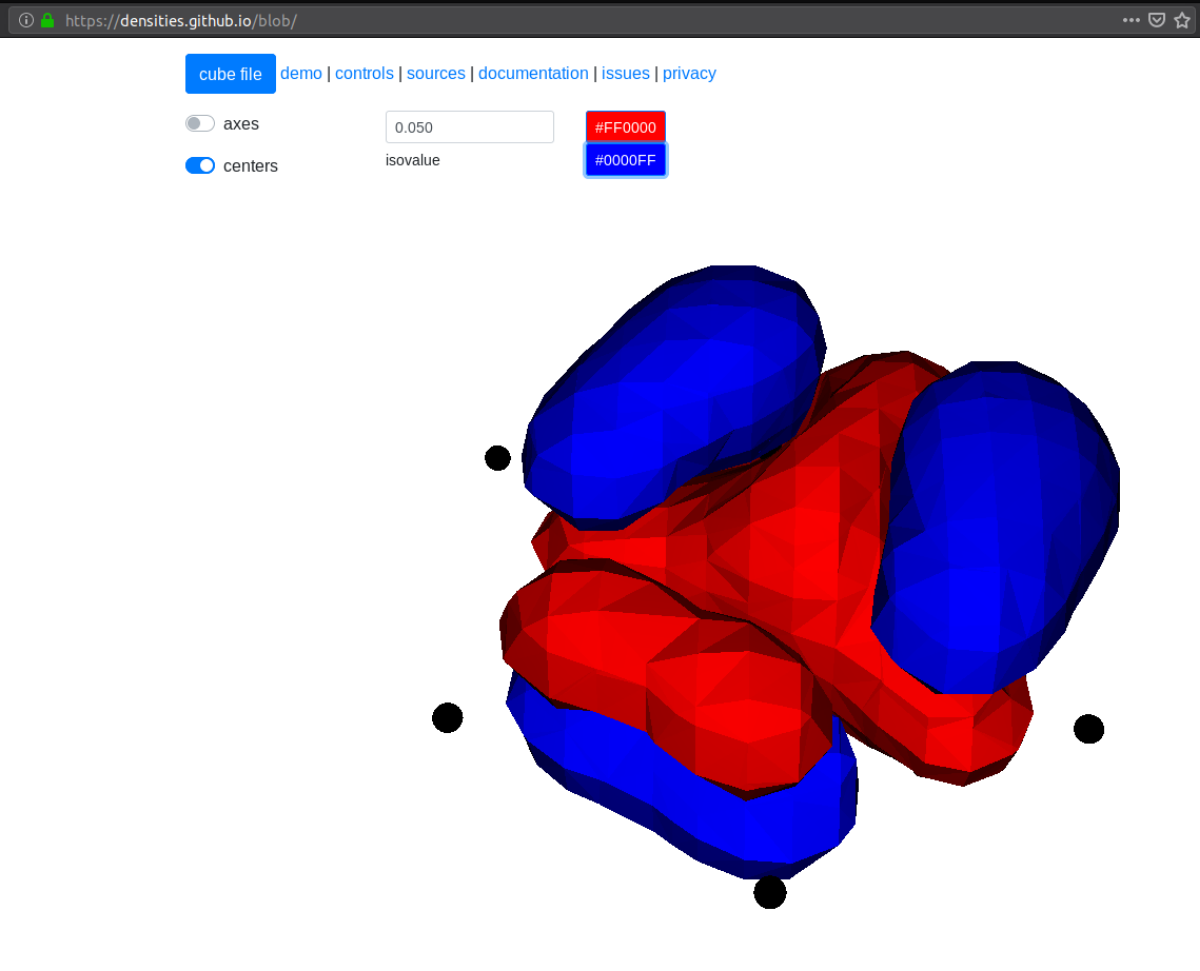
The above example will plot on a 20x20x20 grid in the volume [-4,4]^3, and the generated files (e.g. plots/phi_1_re.cube) can be viewed directly in a web browser by blob , like this benzene orbital:

SCF¶

This section specifies the parameters for the SCF optimization of the ground state wavefunction.

SCF solver¶

The optimization is controlled by the following keywords (defaults shown):

SCF {
  run = true                            # Run SCF solver
  kain = 5                              # Length of KAIN iterative subspace
  max_iter = 100                        # Maximum number of SCF iterations
  rotation = 0                          # Iterations between diagonalize/localize
  localize = false                      # Use canonical or localized  orbitals
  start_prec = -1.0                     # Dynamic precision, start value
  final_prec = -1.0                     # Dynamic precision, final value
  orbital_thrs = 10 * world_prec        # Convergence threshold orbitals
  energy_thrs = -1.0                    # Convergence threshold energy
}

If run = false no SCF is performed, and the properties are computed directly on the initial guess wavefunction.

The kain (Krylov Accelerated Inexact Newton) keyword gives the length of the iterative subspace accelerator (similar to DIIS). The rotation keyword gives the number of iterations between every orbital rotation, which can be either localization or diagonalization, depending on the localize keyword. The first two iterations in the SCF are always rotated, otherwise it is controlled by the rotation keyword (usually this is not very important, but sometimes it fails to converge if the orbitals drift too far away from the localized/canonical forms).

The dynamic precision keywords control how the numerical precision is changed throughout the optimization. One can choose to use a lower start_prec in the first iterations which is gradually increased to final_prec (both are equal to world_prec by default). Note that lower initial precision might affect the convergence rate.

In general, the important convergence threshold is that of the orbitals, and by default this is set one order of magnitude higher than the overall world_prec. For simple energy calculations, however, it is not necessary to converge the orbitals this much due to the quadratic convergence of the energy. This means that the number of correct digits in the total energy will be saturated well before this point, and one should rather use the energy_thrs keyword in this case in order to save a few iterations.

Note

It is usually not feasible to converge the orbitals beyond the overall precision world_prec due to numerical noise.

Initial guess¶

Several types of initial guess are available:

core and sad requires no further input and computes guesses from scratch.

chk and mw require input files from previous MW calculations.

cube requires input files computed from other sources.

The core and sad guesses are computed by diagonalizing the Hamiltonian matrix using a Core or Superposition of Atomic Densities (SAD) Hamiltonian, respectively. The matrix is constructed in a small AO basis with a given “zeta quality”, which should be added as a suffix in the keyword. Available AO bases are hydrogenic orbitals of single sz, double dz, triple tz and quadruple qz zeta size.

The SAD guess can also be computed in a small GTO basis (3-21G), using the guess type sad_gto. In this case another input keyword guess_screen becomes active for screening in the MW projection of the Gaussians. The screening value is given in standard deviations. Such screening will greatly improve the efficiency of the guess for large systems. It is, however, not recommended to reduce the value much below 10 StdDevs, as this will have the opposite effect on efficiency due to introduction of discontinuities at the cutoff point, which leads to higher grid refinement. sad_gto is usually the preferred guess both for accuracy and efficiency, and is thus the default choice.

The core and sad guesses are fully specified with the following keywords (defaults shown):

SCF {
  guess_prec = 1.0e-3                   # Numerical precision used in guess
  guess_type = sad_gto                  # Type of inital guess (chk, mw, cube, core_XX, sad_XX)
  guess_screen = 12.0                   # Number of StdDev before a GTO is set to zero (sad_gto)
}

Checkpointing¶

The program can dump checkpoint files at every iteration using the write_checkpoint keyword (defaults shown):

SCF {
  path_checkpoint = checkpoint          # Path to checkpoint files
  write_checkpoint = false              # Save checkpoint files every iteration
}

This allows the calculation to be restarted in case it crashes e.g. due to time limit or hardware failure on a cluster. This is done by setting guess_type = chk in the subsequent calculation:

SCF {
  guess_type = chk                      # Type of inital guess (chk, mw, cube, core_XX, sad_XX)
}

In this case the path_checkpoint must be the same as the previous calculation, as well as all other parameters in the calculation (Molecule and Basis in particular).

Write orbitals¶

The converged orbitals can be saved to file with the write_orbitals keyword (defaults shown):

SCF {
  path_orbitals = orbitals              # Path to orbital files
  write_orbitals = false                # Save converged orbitals to file
}

This will make individual files for each orbital under the path_orbitals directory. These orbitals can be used as starting point for subsequent calculations using the guess_type = mw initial guess:

SCF {
  guess_prec = 1.0e-3                   # Numerical precision used in guess
  guess_type = mw                       # Type of inital guess (chk, mw, cube, core_XX, sad_XX)
}

Here the orbitals will be re-projected onto the current MW basis with precision guess_prec. We also need to specify the paths to the input files:

Files {
  guess_phi_p = initial_guess/phi_p     # Path to paired MW orbitals
  guess_phi_a = initial_guess/phi_a     # Path to alpha MW orbitals
  guess_phi_b = initial_guess/phi_b     # Path to beta MW orbitals
}

Note that by default orbitals are written to the directory called orbitals but the mw guess reads from the directory initial_guess (this is to avoid overwriting the files by default). So, in order to use MW orbitals from a previous calculation, you must either change one of the paths (SCF.path_orbitals or Files.guess_phi_p etc), or manually copy the files between the default locations.

Note

The mw guess must not be confused with the chk guess, although they are similar. The chk guess will blindly read in the orbitals that are present, regardless of the current molecular structure and computational setup (if you run with a different computational domain or MW basis type/order the calculation will crash). The mw guess will re-project the old orbitals onto the new computational setup and populate the orbitals based on the new molecule (here the computation domain and MW basis do not have to match).

Response¶

This section specifies the parameters for the SCF optimization of the linear response functions. There might be several independent response calculations depending on the requested properties, e.g.

Polarizability {
  frequency = [0.0, 0.0656]             # List of frequencies to compute
}

will run one response for each frequency (each with three Cartesian components), while

Properties {
  magnetizability = true                # Compute magnetizability
  nmr_shielding = true                  # Compute NMR shieldings
}

will combine both properties into a single response calculation, since the perturbation operator is the same in both cases (unless you choose NMRShielding.nuclear_specific = true, in which case there will be a different response for each nucleus).

Response solver¶

The optimization is controlled by the following keywords (defaults shown):

Response {
  run = [true,true,true]                # Run response solver [x,y,z] direction
  kain = 5                              # Length of KAIN iterative subspace
  max_iter = 100                        # Maximum number of SCF iterations
  localize = false                      # Use canonical or localized  orbitals
  start_prec = -1.0                     # Dynamic precision, start value
  final_prec = -1.0                     # Dynamic precision, final value
  orbital_thrs = 10 * world_prec        # Convergence threshold orbitals
}

Each linear response calculation involves the three Cartesian components of the appropriate perturbation operator. If any of the components of run is false, no response is performed in that particular direction, and the properties are computed directly on the initial guess response functions (usually zero guess).

The kain (Krylov Accelerated Inexact Newton) keyword gives the length of the iterative subspace accelerator (similar to DIIS). The localize keyword relates to the unperturbed orbitals, and can be set independently of the SCF.localize keyword.

The dynamic precision keywords control how the numerical precision is changed throughout the optimization. One can choose to use a lower start_prec in the first iterations which is gradually increased to final_prec (both are equal to world_prec by default). Note that lower initial precision might affect the convergence rate.

For response calculations, the important convergence threshold is that of the orbitals, and by default this is set one order of magnitude higher than the overall world_prec.

Note

The quality of the response property depends on both the perturbed as well as the unperturbed orbitals, so they should be equally well converged.

Initial guess¶

The following initial guesses are available:

none start from a zero guess for the response functions.

chk and mw require input files from previous MW calculations.

By default, no initial guess is generated for the response functions, but the chk and mw guesses work similarly as for the SCF.

Checkpointing¶

The program can dump checkpoint files at every iteration using the write_checkpoint keyword (defaults shown):

Response {
  path_checkpoint = checkpoint          # Path to checkpoint files
  write_checkpoint = false              # Save checkpoint files every iteration
}

This allows the calculation to be restarted in case it crashes e.g. due to time limit or hardware failure on a cluster. This is done by setting guess_type = chk in the subsequent calculation:

Response {
  guess_type = chk                      # Type of inital guess (none, chk, mw)
}

In this case the path_checkpoint must be the same as the previous calculation, as well as all other parameters in the calculation (Molecule and Basis in particular).

Write orbitals¶

The converged response orbitals can be saved to file with the write_orbitals keyword (defaults shown):

Response {
  path_orbitals = orbitals              # Path to orbital files
  write_orbitals = false                # Save converged orbitals to file
}

This will make individual files for each orbital under the path_orbitals directory. These orbitals can be used as starting point for subsequent calculations using the guess_type = mw initial guess:

Response {
  guess_prec = 1.0e-3                   # Numerical precision used in guess
  guess_type = mw                       # Type of inital guess (chk, mw, cube, core_XX, sad_XX)
}

Here the orbitals will be re-projected onto the current MW basis with precision guess_prec. We also need to specify the paths to the input files (only X for static perturbations, X and Y for dynamic perturbations):

Files {
  guess_X_p = initial_guess/X_p         # Path to paired MW orbitals
  guess_X_a = initial_guess/X_a         # Path to alpha MW orbitals
  guess_X_b = initial_guess/X_b         # Path to beta MW orbitals
  guess_Y_p = initial_guess/Y_p         # Path to paired MW orbitals
  guess_Y_a = initial_guess/Y_a         # Path to alpha MW orbitals
  guess_Y_b = initial_guess/Y_b         # Path to beta MW orbitals
}

Note that by default orbitals are written to the directory called orbitals but the mw guess reads from the directory initial_guess (this is to avoid overwriting the files by default). So, in order to use MW orbitals from a previous calculation, you must either change one of the paths (Response.path_orbitals or Files.guess_X_p etc), or manually copy the files between the default locations.